RF (Random Forest)
Contents
RF (Random Forest)#
We will break timeline a bit and jump to random forests instead of introducing perceptrons. The general method of random decision forests was first proposed by Ho only in 1995. RF became really popular approach for tabular dataset due to their simplicity and quite robust behaviour. They are still widely used and for some problems can outperform neural nets.
Before defining random forests we need to explore it’s main building block - entropy.
Entropy#
Coined by Claude Shannon in “A Mathematical Theory of Communication” 1948 (link). Main question: how much useful information are we transmitting? When we transmit one bit of information we reduce recipients uncertainty by the factor of two.
P.S.: same paper introduced term bit = binary unit.
Look at the following video:
Some key points:
How much information are we getting measured in bits? \(- \log_2 (prob) = bits\)
Entropy: \(H(p)=-\sum_i p_i \log_2 (p_i)\)
Cross-Entropy: let \(p\) - true distribution, \(q\) - predicted distribution, then Cross-entropy is \(H(p,q) = -\sum_i p_i \log_2(q_i)\)
If predictions are perfect Cross-entropy is equal to entropy, but usually it is greater than entropy.
Cross-entropy is often used for ML as a cost function (log-loss) comparing \(p\) with \(q\).
%matplotlib inline

import numpy as np
import pandas as pd
from sklearn.datasets import load_iris
import matplotlib.pyplot as plt
from sklearn.tree import DecisionTreeClassifier, export_graphviz
from graphviz import Source
from IPython.display import display, SVG
Iris dataset#
Bellow we will work with iris dataset. The idea of the dataset is to find out iris class based on given measurements.
# Load dataset
iris = load_iris()
df = pd.DataFrame(iris.data, columns = iris.feature_names)
df['class'] = iris.target_names[iris.target]
df
| sepal length (cm) | sepal width (cm) | petal length (cm) | petal width (cm) | class | |
|---|---|---|---|---|---|
| 0 | 5.1 | 3.5 | 1.4 | 0.2 | setosa |
| 1 | 4.9 | 3.0 | 1.4 | 0.2 | setosa |
| 2 | 4.7 | 3.2 | 1.3 | 0.2 | setosa |
| 3 | 4.6 | 3.1 | 1.5 | 0.2 | setosa |
| 4 | 5.0 | 3.6 | 1.4 | 0.2 | setosa |
| ... | ... | ... | ... | ... | ... |
| 145 | 6.7 | 3.0 | 5.2 | 2.3 | virginica |
| 146 | 6.3 | 2.5 | 5.0 | 1.9 | virginica |
| 147 | 6.5 | 3.0 | 5.2 | 2.0 | virginica |
| 148 | 6.2 | 3.4 | 5.4 | 2.3 | virginica |
| 149 | 5.9 | 3.0 | 5.1 | 1.8 | virginica |
150 rows × 5 columns
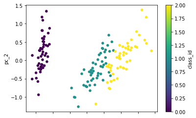
We have 4 dimensions, but we already know that we can visualize that using PCA.
from sklearn.decomposition import PCA
pca = PCA(2)
pca.fit(df.drop('class', axis=1))
PCA(n_components=2)
X = pca.transform(df.drop('class', axis=1))
pc = pd.DataFrame(X, columns=['pc_1', 'pc_2'])
pc['class_id'] = iris.target

pc.plot(kind='scatter', x='pc_1', y='pc_2', c='class_id', cmap='viridis')
<AxesSubplot:xlabel='pc_1', ylabel='pc_2'>
Decision Trees#
Simple decision tree can be constructed using rule: make a split which reduces entropy the most. In a well-constructed tree, each question will cut the number of options by approximately half, very quickly narrowing the options even among a large number of classes.

Couple facts about decision trees:
Alternatively you could use Gini impurity as a split criteria, which is defined as \(G_i = 1 - \sum_{k=1}^n p_{i,k}^2\) where \(p_{i,k}\) is the ratio of class k instances among the training instances in the ith node.
Finding the optimal tree is known to be an NP-Complete problem \(O(\exp (m))\).
Decision Trees are very sensitive to small variations in the training data.
Decision Trees can easily over-fit if there is high number of columns!
Let’s try this out on iris dataset. First we will need to make train/test split.
from sklearn.model_selection import train_test_split

X_train, X_test, y_train, y_test = train_test_split(
    df.drop('class', axis=1), df['class'],
    test_size=0.3, random_state=42)
Let’s fit entropy based tree on iris dataset.
for max_depth in range(1, 4):
    print('-' * 70 + '\nTree for max_dept = {0}\n'.format(max_depth))
    tree = DecisionTreeClassifier(max_depth=max_depth, criterion='entropy')
    # Fit on train data
    tree.fit(X_train, y_train)

    # Make prediction and evaluate performance
    pred_train = tree.predict(X_train)
    pred_test = tree.predict(X_test)
    print('Correctly identified on train set - {0:.02%}, on test set - {1:.02%}'.format(
        (pred_train == y_train).mean(),
        (pred_test == y_test).mean()))

    # Make a nice plot
    graph = Source(export_graphviz(tree, out_file=None, filled = True,
                                   feature_names=df.drop('class', axis=1).columns,
                                   class_names=['0 - setosa', '1 - versicolor', '2 - virginica']))
    display(SVG(graph.pipe(format='svg')))
----------------------------------------------------------------------
Tree for max_dept = 1

Correctly identified on train set - 64.76%, on test set - 71.11%

----------------------------------------------------------------------
Tree for max_dept = 2

Correctly identified on train set - 94.29%, on test set - 100.00%

----------------------------------------------------------------------
Tree for max_dept = 3

Correctly identified on train set - 95.24%, on test set - 97.78%

As we can see simple decision tree works quite good for iris dataset.
Larger dataset and overfit example#
Let’s load another legendary dataset containing classification problem. If you are interested in dataset details see UCI.
from sklearn.datasets import load_breast_cancer

# Load dataset
cancer = load_breast_cancer()
df = pd.DataFrame(cancer.data, columns = cancer.feature_names)
df['class'] = cancer.target_names[cancer.target]

# Train/test split
X_train, X_test, y_train, y_test = train_test_split(
    df.drop('class', axis=1), df['class'],
    test_size=0.4, random_state=42)
df.groupby('class').size()
class
benign       357
malignant    212
dtype: int64
As before we will fit multiple trees with different max_depth’s. This time let’s plot performance on train and test sets.
L = []
for max_depth in range(1, 10):
    tree = DecisionTreeClassifier(max_depth=max_depth, criterion='entropy', random_state=42)
    # Fit on train data
    tree.fit(X_train, y_train)

    # Make prediction and evaluate performance
    pred_train = tree.predict(X_train)
    pred_test = tree.predict(X_test)
    L.append([(pred_train == y_train).mean(),
              (pred_test == y_test).mean()])

pd.DataFrame(L, columns=['train', 'test']).plot(
    title='Accuracy for different max_depth values')
<AxesSubplot:title={'center':'Accuracy for different max_depth values'}>
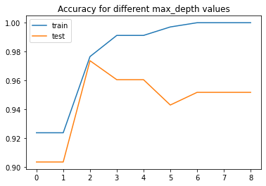
Notice that as the depth increases, we tend to get very strangely shaped classification regions. Such overfitting turns out to be a general property of decision trees: it is very easy to go too deep in the tree, and thus to fit details of the particular data rather than the overall properties of the distributions they are drawn from. Another way to see this overfitting is to look at models trained on different subsets of the data.
How can we prevent it in this case?
Ensembles#
The notion that multiple overfitting estimators can be combined to reduce the effect of overfitting is what underlies an ensemble method called bagging. Bagging makes use of an ensemble (a grab bag, perhaps) of parallel estimators, each of which overfits the data, and averages the results to find a better classification. An ensemble of randomized decision trees is known as a random forest.


Ensemble methods work best when the predictors are as independent from one another as possible. One way to get diverse classifiers is to train them using very different algorithms. This increases the chance that they will make very different types of errors, improving the ensemble’s accuracy.
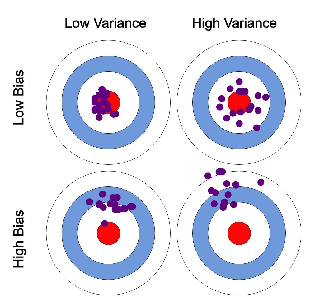
Ensemble methods lead to similar bias but a lower variance.
Random forests#
You can make multiple trees by choosing sub-sample of features (usually \(\sqrt{m}\)) and taking bootstrapped samples. Then just let trees vote for decision.
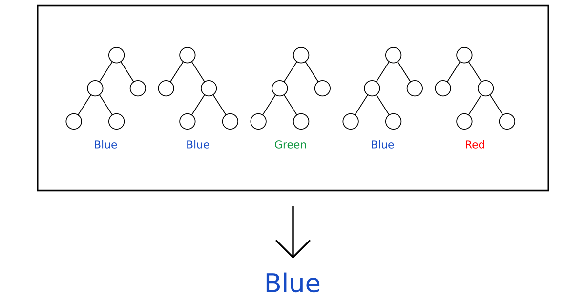
Hard voting averages predictions, soft voting averages predicted probabilities instead.
from sklearn.ensemble import BaggingClassifier

# Defining the base estimator
base = DecisionTreeClassifier(max_depth=5, splitter='best',
                              max_features='sqrt', criterion='entropy')

# Create Random Forest
ensemble = BaggingClassifier(base_estimator=base, n_estimators=1000,
                             bootstrap=True)
%%time

ensemble.fit(X_train, y_train)
pred_train = ensemble.predict(X_train)
pred_test = ensemble.predict(X_test)

print('Correctly identified on train set - {0:.02%}, on test set - {1:.02%}\n'.format(
    (pred_train == y_train).mean(),        # train set
    (pred_test == y_test).mean()))         # test set
Correctly identified on train set - 99.71%, on test set - 96.93%

CPU times: user 1.19 s, sys: 311 ms, total: 1.5 s
Wall time: 830 ms
In realiy you should use RandomForestClassifier implementation instead. Lines above are only for illustation purposes.
from sklearn.ensemble import RandomForestClassifier
RandomForestClassifier?
%%time

rf = RandomForestClassifier(1000, criterion='entropy', max_depth=10)
rf.fit(X_train, y_train)
pred_train = rf.predict(X_train)
pred_test = rf.predict(X_test)

print('Correctly identified on train set - {0:.02%}, on test set - {1:.02%}\n'.format(
    (pred_train == y_train).mean(),
    (pred_test == y_test).mean()))
Correctly identified on train set - 100.00%, on test set - 97.81%

CPU times: user 736 ms, sys: 11.6 ms, total: 747 ms
Wall time: 753 ms
Note: there are other variations of boosted trees, for example ExtraTrees can be constructed by setting splitter to random and bootstrap to False. ExtraTrees are usually faster to train, but Random Forests are more well known, just try them both and see which works better for problem at hand.
Task#
Try to use sklearn.ensemble.RandomForestClassifier for iris dataset. Use sklearn implementation.
# Load dataset
iris = load_iris()
df = pd.DataFrame(iris.data, columns = iris.feature_names)
df['class'] = iris.target_names[iris.target]

# df['sepal area'] = df['sepal length (cm)'] * df['sepal width (cm)']
# df['petal area'] = df['petal length (cm)'] * df['petal width (cm)']
# df['visual pleasure'] = df['sepal area'] / df['petal area']

# Train/test split
X_train, X_test, y_train, y_test = train_test_split(
    df.drop(['class', 'sepal length (cm)', 'sepal width (cm)',
             'petal length (cm)', 'petal width (cm)'], axis=1), df['class'],
    test_size=0.5, random_state=42)

# TODO:
# 1. train RF and compare results to the ones we had above
# 2. add more features
rf = RandomForestClassifier(1000, criterion='entropy', max_depth=10)
rf.fit(X_train, y_train)
pred_train = rf.predict(X_train)
pred_test = rf.predict(X_test)
---------------------------------------------------------------------------
ValueError                                Traceback (most recent call last)
/var/folders/71/2t6j6ytn1t3dfp5dxb9zhh6w0000gn/T/ipykernel_22584/4229513911.py in <module>
      1 rf = RandomForestClassifier(1000, criterion='entropy', max_depth=10)
----> 2 rf.fit(X_train, y_train)
      3 pred_train = rf.predict(X_train)
      4 pred_test = rf.predict(X_test)

/opt/homebrew/Caskroom/miniforge/base/envs/ai_primer/lib/python3.9/site-packages/sklearn/ensemble/_forest.py in fit(self, X, y, sample_weight)
    301                 "sparse multilabel-indicator for y is not supported."
    302             )
--> 303         X, y = self._validate_data(X, y, multi_output=True,
    304                                    accept_sparse="csc", dtype=DTYPE)
    305         if sample_weight is not None:

/opt/homebrew/Caskroom/miniforge/base/envs/ai_primer/lib/python3.9/site-packages/sklearn/base.py in _validate_data(self, X, y, reset, validate_separately, **check_params)
    430                 y = check_array(y, **check_y_params)
    431             else:
--> 432                 X, y = check_X_y(X, y, **check_params)
    433             out = X, y
    434

/opt/homebrew/Caskroom/miniforge/base/envs/ai_primer/lib/python3.9/site-packages/sklearn/utils/validation.py in inner_f(*args, **kwargs)
     70                           FutureWarning)
     71         kwargs.update({k: arg for k, arg in zip(sig.parameters, args)})
---> 72         return f(**kwargs)
     73     return inner_f
     74

/opt/homebrew/Caskroom/miniforge/base/envs/ai_primer/lib/python3.9/site-packages/sklearn/utils/validation.py in check_X_y(X, y, accept_sparse, accept_large_sparse, dtype, order, copy, force_all_finite, ensure_2d, allow_nd, multi_output, ensure_min_samples, ensure_min_features, y_numeric, estimator)
    793         raise ValueError("y cannot be None")
    794
--> 795     X = check_array(X, accept_sparse=accept_sparse,
    796                     accept_large_sparse=accept_large_sparse,
    797                     dtype=dtype, order=order, copy=copy,

/opt/homebrew/Caskroom/miniforge/base/envs/ai_primer/lib/python3.9/site-packages/sklearn/utils/validation.py in inner_f(*args, **kwargs)
     70                           FutureWarning)
     71         kwargs.update({k: arg for k, arg in zip(sig.parameters, args)})
---> 72         return f(**kwargs)
     73     return inner_f
     74

/opt/homebrew/Caskroom/miniforge/base/envs/ai_primer/lib/python3.9/site-packages/sklearn/utils/validation.py in check_array(array, accept_sparse, accept_large_sparse, dtype, order, copy, force_all_finite, ensure_2d, allow_nd, ensure_min_samples, ensure_min_features, estimator)
    531
    532         if all(isinstance(dtype, np.dtype) for dtype in dtypes_orig):
--> 533             dtype_orig = np.result_type(*dtypes_orig)
    534
    535     if dtype_numeric:

<__array_function__ internals> in result_type(*args, **kwargs)

ValueError: at least one array or dtype is required
np.mean(pred_train == y_train)
np.mean(pred_test == y_test)
pd.DataFrame(rf.feature_importances_[np.newaxis],
             columns=df.drop(['class', 'sepal length (cm)', 'sepal width (cm)',
             'petal length (cm)', 'petal width (cm)'], axis=1).columns).T.sort_values(0).style.background_gradient()
I suggest to try it out on your own before looking at the answer given bellow.
Possible answer#
from sklearn.ensemble import RandomForestClassifier
df['sepal area'] = df['sepal length (cm)'] * df['sepal width (cm)']
df['petal area'] = df['petal length (cm)'] * df['petal width (cm)']
df['simetry'] = df['sepal area'] / df['petal area']
X_train, X_test, y_train, y_test = train_test_split(
    df.drop('class', axis=1), df['class'],
    test_size=0.5, random_state=42)
rf = RandomForestClassifier(n_estimators=1000, max_depth=2)
rf.fit(X_train, y_train)
pred = rf.predict(X_test)
acc = np.mean(pred == y_test)
print(f'Accuracy {acc:.02%}')
Neat tricks#
Confusion matrix#
Thisis a neat way to see where your model is making mistakes.
from sklearn.metrics import confusion_matrix
pd.DataFrame(confusion_matrix(y_test, pred),
             columns=rf.classes_, index=rf.classes_).style.background_gradient()
Feature importance#
It is easy to check which features are most important - ones which were used in most trees or/and gave highest information gain overall.
pd.DataFrame(rf.feature_importances_,
             index=df.drop('class', axis=1).columns).style.background_gradient()
A note on decision boundaries#
Let’s generate some data blobs.
from sklearn.tree import DecisionTreeClassifier
from sklearn.ensemble import RandomForestClassifier
from sklearn.datasets import make_blobs

X, y = make_blobs(n_samples=300, centers=4,
                  random_state=0, cluster_std=1.0)

tree = DecisionTreeClassifier()
tree.fit(X, y)

rf = RandomForestClassifier(n_estimators=500, max_depth=2)
rf.fit(X, y)
Look at overfitting here, make decision boundary plots.
mesh = np.transpose([np.tile(np.linspace(-5, 5, 100), 100),
                     np.repeat(np.linspace(-3, 12, 100), 100)])

plt.figure(figsize=(16, 8))
plt.subplot(121)
plt.scatter(mesh[:, 0], mesh[:, 1], c=tree.predict(mesh), marker='s', s=20, cmap='inferno')
plt.scatter(X[:, 0], X[:, 1], c=y, cmap='coolwarm')
plt.title('Simple decision tree')
plt.subplot(122)
plt.scatter(mesh[:, 0], mesh[:, 1], c=rf.predict(mesh), marker='s', s=20, cmap='inferno')
plt.scatter(X[:, 0], X[:, 1], c=y, cmap='coolwarm')
plt.title('Random forest')
plt.show()
Make sure that you understand why those decision boundaries look this way.
By the way, RF with standard param set will not look so nice, play around.
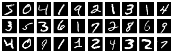
MNIST#
The MNIST database contains handwritten digits and has a training set of 60,000 examples, and a test set of 10,000 examples. It is legendary dataset crated by LeCun group in 1999.
from tensorflow import keras

(X_train, y_train), (X_test, y_test) = keras.datasets.mnist.load_data()
# Normalize
X_train = X_train / 255
X_test = X_test / 255

plt.figure(figsize=(10, 3))
for i in range(30):
    plt.subplot(3, 10, i + 1)
    plt.imshow(X_train[i], cmap='gray')
    plt.axis('off')
plt.show()

X_train = X_train.reshape((60000, 28*28))
X_test = X_test.reshape((10000, 28*28))
Init Plugin
Init Graph Optimizer
Init Kernel
model = RandomForestClassifier()
model.fit(X_train, y_train)
pred = model.predict(X_test)
from sklearn.metrics import accuracy_score

accuracy_score(y_test, pred)
0.9694
import pandas as pd
from sklearn.metrics import confusion_matrix

pd.DataFrame(confusion_matrix(y_test, pred), columns=range(10), index=range(10)).style.background_gradient()
| 0 | 1 | 2 | 3 | 4 | 5 | 6 | 7 | 8 | 9 | |
|---|---|---|---|---|---|---|---|---|---|---|
| 0 | 970 | 0 | 0 | 0 | 0 | 3 | 3 | 1 | 2 | 1 |
| 1 | 0 | 1124 | 2 | 4 | 0 | 1 | 3 | 0 | 1 | 0 |
| 2 | 6 | 0 | 1002 | 5 | 2 | 0 | 2 | 10 | 5 | 0 |
| 3 | 0 | 0 | 10 | 972 | 0 | 7 | 0 | 10 | 9 | 2 |
| 4 | 1 | 0 | 2 | 0 | 958 | 0 | 5 | 0 | 3 | 13 |
| 5 | 2 | 1 | 1 | 17 | 2 | 856 | 4 | 2 | 5 | 2 |
| 6 | 5 | 3 | 0 | 0 | 5 | 5 | 936 | 0 | 4 | 0 |
| 7 | 1 | 2 | 20 | 3 | 2 | 0 | 0 | 988 | 2 | 10 |
| 8 | 4 | 0 | 5 | 6 | 6 | 7 | 4 | 4 | 927 | 11 |
| 9 | 7 | 5 | 3 | 9 | 13 | 1 | 1 | 5 | 4 | 961 |
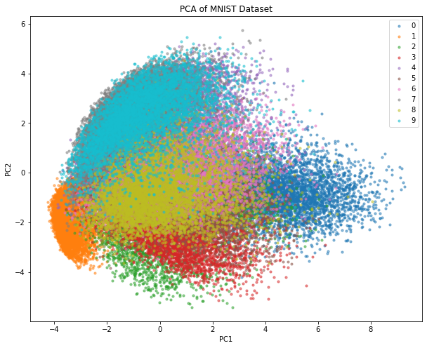
TASK: using PCA compress MNIST to two dimensions and make a plot (color by class label).
# Reshape the data from 28x28 to 784
X_train_flat = X_train.reshape(-1, 28*28)

# Apply PCA and reduce the dimensionality to 2
pca = PCA(n_components=2)
X_train_pca = pca.fit_transform(X_train_flat)

# Plot the data
plt.figure(figsize=(10, 8))
for i in range(10):  # there are 10 classes (0 to 9) in MNIST
    subset = X_train_pca[y_train == i]
    plt.scatter(subset[:, 0], subset[:, 1], label=str(i), alpha=0.5, s=10)

plt.legend()
plt.xlabel("PC1")
plt.ylabel("PC2")
plt.title("PCA of MNIST Dataset")
plt.show()
True labels are on the left and predicted ones on the top. Quick glimpse gives you insightes like - RF makes most mistakes while identifying actual 7 as 2 and actual 4 as 9. What other insights can you give?
Soon we will see that using neural networks we can avoid some of these mistakes, but key insight here is that RF is good method even for complex tasks as this one.
Whats next?#
There are many variations of Random Forests you can explore, to name a few:
Up to the day of writing XGboost is still a leading method for tabular problems, but as we will see deep learning will beat them at unstructured data. Basic idea of XGBoost: fit next decision tree on residual errors made by the previous predictor, thus trying to fix them.
Fit \(\text{tree}_0\) on \(X\) and \(y_0=y\) and make predictions \(y_1\). Set \(i=1\).
Fit \(\text{tree}_i\) to predict residuals \(y_{i-1} - y_i\) given \(X\) and make predictions \(y_{i+1}\).
Increment \(i\) and jump back to step 2.